- Fatigue Technologies
- Constant Amplitude
- Variable Amplitude
- Finite Element Model
- Fatigue Analyzers
- Finders
- Technical Background
- Multiaxial
- Probabilistic
- High Temperature
- Welded Structures
- Cast Iron
- Small Defect √ Area
- Utilities
- Languages
 日本語
日本語eFatigue gives you everything you need to perform state-of-the-art fatigue analysis over the web. Click here to learn more about eFatigue.
Finite Element Model Strain-Life Technical Background
In order to accurately assess fatigue lives from finite element models consideration must be given to multiaixal stresses, stress gradients and variable amplitude out-of-phase loading in addition to traditional factors such as surface finish and mean stresses.
Almost all fatigue data are reported in terms of tensile stress for constant amplitude uniaxial loading, i.e. the SN or εN material curves. But, the state of stress and strain are usually multiaxial in any structure or component. A multiaxial fatigue analysis is needed to relate the more complex stress state found in all structures and components to the simple stress state used for material testing. What stress, or strain, should be used as the basis of comparison, principle, shear or von Mises equivalent? Fatigue crack nucleation and early growth is a process that is driven by shear stresses. Once nucleated, a crack tends to grow in perpendicular to the maximum principle stress direction. As a result, two fatigue damage models must always be used to accurately assess fatigue lives. One that considers the possibility of shear stress/strain dominated failures and a second one that considers principle stress/strain failure mechanisms.
Stress and strain gradient effects also play an important role in accurately assessing fatigue damage. Small notch or stress concentration features or geometries with high stress gradients are less effective in fatigue than larger features or smaller gradients with the same maximum stress. In conventional fatigue analysis, the stress gradient effect is taken into account by using a fatigue notch factor, Kf, rather than the stress concentration factor Kt. In practice Kf < Kt. Since there is no concept of a Kt or nominal stress in a finite element model stress gradient effects are considered directly. In conventional fatigue analysis, Kt gives the stress on the surface and Kf gives a lower stress just below the surface. In a finite element model it is easy to compute the stress at any distance below the surface. Typically this distance is 0.5 mm. The method is described in the literature as the critical distance method.
Performing a variable amplitude multiaxial fatigue analysis with stress gradient effects on every node or element is too time consuming to be practical. Methods have been devised to screen out those elements and nodes with little or no fatigue damage. Fatigue is a surface phenomena where fatigue cracks start. Only those nodes and elements on the surface are considered substantially reducing the number of nodes to be analyzed. Next those nodes and elements with stresses too small to cause any fatigue damage are eliminated. The result of this screening is a manageable number of nodes and elements, each of which is treated as a potential variable amplitude multiaxial fatigue problem.
Theories
Theories and equations employed in the eFatigue FEM Strain-Life Analyzer are described in this section. A description of the input and output options are given in the next section.
Plasticity Correction
eFatigue assumes an elastic finite element model is used as the input.
In uniaxial loading approximate solutions such as Neuber's rule are used to compute the stresses and strains during plastic deformation. Unfortunately, Neuber's rule cannot be directly extended to multiaxial loading because there are six unknowns and only five equations.
To overcome this problem Koettgen et al. (Koettgen V.B., Barkey M.E., and Socie, D.F. "Pseudo Stress and Pseudo Strain Based Approaches to Multiaxial Notch Analysis" Fatigue and Fracture of Engineering Materials and Structures, Vol. 18, No. 9, 1995, 981-1006) proposed a structural yield surface to obtain local elastic-plastic stresses and strains. Having defined a "yield surface," standard cyclic plasticity methods can be used to solve for the unknown stresses and strains at the notch. The material memory effects are built directly into standard cyclic plasticity calculations. The method is based on the same concept at the analytical or experimental nominal stress - notch strain curves used in uniaxial fatigue analysis such as the one shown here.
Nominal stress - notch strain curve
Cyclically, nominal stress - notch root strain response has all the features associated with stress-strain response such as hysteresis, memory, cyclic hardening and softening.
Next we introduce the concept of pseudo stress. The pseudo stress, es, or strain, ee, is defined as the theoretical elastic stress or strain computed using elastic assumptions. Neuber's rule may be written in terms of pseudo stress as follows.


These concepts can be generalized to three dimensional stress and strain states with a structural yield surface at a notch. Having defined a "structural yield surface," standard cyclic plasticity methods can be used to solve for the unknown stresses and strains at the notch. For multiaxial loading, the total stress or strain is obtained by superposition of the individual load cases.
A relationship between pseudo stress and notch strain is described with a power function that has the same form as a stress-strain curve
where the constants K* and n* represent the behavior of the structure rather than the material. Uniaxial Neuber's rule can be employed to establish the constants E*, K* and n*.
For plane stress on the surface, eσz, eτyz and eτxz are all zero and this yield function can be written as
This equation defines a structural yield function, Fo, which has the same form as the yield functions used in the plasticity models for stress-strain calculations, i.e. a Mises yield function in terms of pseudo stress.

The process may be summarized as follows:
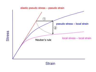
- uniaxial Neuber's rule to get K* and n*
- 1. cyclic plasticity model in stress control with pseudo constants K* and n* to obtain the pseudo stress-local strain response
- 2. cyclic plasticity model in strain control with material constants K and n to obtain the local strain - local stress response.
Go to the Multiaxial Technical Background section for a more complete description of the cyclic plasticity model.
Multiaxial Fatigue Models
No single fatigue theory is applicable for all materials. Some materials tend to form small microcracks during the first loading cycles. These microcracks then grow in a direction perpendicular to the maximum principle stress. Other more ductile materials tend to form shear microcracks. As a result two damage models are used in eFatigue.
Tensile Damage Model
A damage model is needed for materials that fail predominantly by microcrack growth on planes of maximum tensile strain or stress, for example, cast iron, very high strength steels or 304 stainless steel under some local histories. In these materials, cracks nucleate in shear, but fatigue life is controlled by crack growth on planes perpendicular to the maximum principal stress and strain as illustrated below. Both strain range and maximum stress determine the amount of fatigue damage.
Smith et al. (Smith, R.N., Watson, P., and Topper, T.H., "A Stress-Strain Parameter for the Fatigue of Metals," Journal of Materials, Vol. 5, No. 4, 1970, 767-778 proposed a suitable relationship that includes both the cyclic strain range and the maximum stress. This model, commonly referred to as the SWT parameter, was originally developed and continues to be used as a correction for mean stresses in uniaxial loading situations. The SWT parameter is used in the analysis of both proportionally and nonproportionally loaded components for materials that fail primarily due to mode I tensile cracking. The SWT parameter for multiaxial loading is based on the principal strain range, Δε1 and maximum stress on the principal strain range plane, σn,max.
The stress term in this model makes it suitable for describing mean stresses during multiaxial loading and nonproportional hardening effects.
Shear Damage Model
Fatemi and Socie (Fatemi, A. and Socie, D.F., "A Critical Plane Approach to Multiaxial Fatigue Damage Including Out-of-Phase Loading," Fatigue and Fracture of Engineering Materials and Structures, Vol. 11, No. 3, 1988, 149-166) built on the work of Brown and Miller but suggested that the normal strain term should be replaced by the normal stress. The conceptual basis for a damage model is shown below.
During shear loading, the irregularly shaped crack surface results in frictional forces that will reduce crack tip stresses, thus hindering crack growth and increasing the fatigue life. Tensile stresses and strains will separate the crack surfaces and reduce frictional forces. Fractographic evidence for this behavior has been obtained. Fractographs from specimens that have failed by pure torsion show extensive rubbing and are relatively featureless in contrast to tension test fractographs where individual slip bands are observed on the fracture surface.
Extensive experimental observations lead to the following damage model that may be interpreted as the cyclic shear strain modified by the normal stress to include the crack closure effects.
The sensitivity of a material to normal stress is reflected in the value k/σy. As a first approximation or if test data from multiple stress states is not available, k = 0.3. This model not only explains the difference between tension and torsion loading but also can be used to describe mean stress and nonproportional hardening effects. Critical plane models that include only strain terms cannot reflect the effect of mean stress or strain path dependent on hardening.
Go to the Multiaxial Technical Background section for a more complete description of the fatigue analysis.
Surface Finish Effects
Materials, as they are tested, are always in a different surface condition than the materials as they are actually used. Test specimens are polished to eliminate the effects of surface finish. Fatigue cracks usually nucleate on the surface so that the condition of the surface plays a major role in the fatigue resistance of a component, but only at long lives. At short lives cyclic plasticity dominates the behavior of the material and surface finish is less important. The degree of surface damage depends not only on the processing but also on the strength of the material. Higher strength materials are more susceptible to surface damage. An important part of the analysis is to "correct" the basic materials data to obtain an estimate of the fatigue life of the material in the component or structure of interest. To account for this in the analysis the material fatigue limit is reduced by a surface finish factor, kSF.
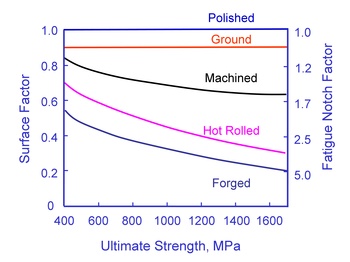
The original data for constructing this curve is shown below. The factors tend to provide conservative estimates for fatigue lives.
(From Noll and Lipson, "Allowable Working Stresses", Society for Experimental Stress Analysis, Vol. III, no. 2, 1949)
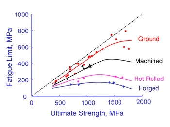
These data are fit to a simple power function to obtain an estimate of the surface factor for any hardness steel.

| α | β | |
| Ground | 1.58 | -0.085 |
| Machined | 4.51 | -0.265 |
| Hot Rolled | 57.7 | -0.718 |
| Forged | 272 | -0.995 |
The effect of surface finish is reduced for higher strain levels where cyclic plasticity controls the behavior. Surface finish won't have any effect on the static strength of the material ( 1 reversal ).
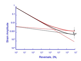
Surface finish effects are included in the analysis by altering the slope of the elastic portion of the strain-life curve. The surface finish corrected slope is given by
It is important to note that this correction should be done after the cyclic strength properties are determined.
Stress Gradient Effects
Small stress concentration features or geometries with high stress gradients are less effective in fatigue than larger features or smaller gradients with the same maximum stress. A plate with a small hole, say 0.1mm, will have a much longer fatigue life than one with a large hole of 10mm even though both plates have the same stress concentration factor and maximum stress. In conventional fatigue analysis, the stress gradient effect is taken into account by using a emperical fatigue notch factor, Kf, rather than the stress concentration factor Kt. Since there is no concept of a Kt or nominal stress in a finite element model stress gradient effects are considered directly. The figure below shows the stress distribution in a plate for three different hole sizes. All of the holes have the same maximum stress, three times the nominal stress.
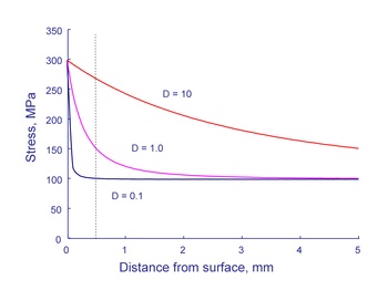
The figure shows that the stresses are independent of size only at the edge of the hole and very far from the hole. The dashed line in the figure is drawn at 0.5mm. Here the stresses increase as the size of the hole increases. Suppose crack nucleation mechanisms result in a crack with a size of 0.5mm. For the smallest hole, 0.1mm, the stress available for continued growth is only 100MPa, the nominal stress. The same size crack is subjected to a stress of 275 MPa in the larger hole, nearly equal to the maximum stress.
What about the nucleation of a crack around a hole of different sizes? It is useful to think about a process zone for crack nucleation. Materials are not continuous and homogeneous on the size scale that crack nucleation mechanisms operate. The grain size of the material is a convienient way to visualize the fatigue process zone. The figure below shows the grain size superimposed on the stress distribution from the figure above. What is the stress in the process zone? A simple first approximation would be to take the stress in the center of the grain. Thus, a stress of 275MPa would be used to compute the fatigue life of a 10mm hole and a stress of 100MPa would be used for the 0.1mm hole.
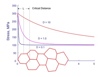
The modern view of fatigue is that when a material is stressed at the fatigue limit a microcrack will form but not grow outside of the process zone. Stresses gradient effects are included in the fatigue analysis in a very simple and straightforward manner. Stresses and strains at a distance L/2 from the surface are used rather than the surface stresses and strains.
The critical distance can be expressed in terms of the threshold stress intensity, ΔKTH, and fatigue limit range, ΔσFL, as
Computing the critical distance from the threshold stress intensity is difficult because the threshold stress intensity, particularly for small microcracks, is usually unknown. Fortunately there is a good direct correlation between the critical distance and fatigue limit.
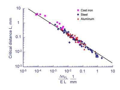
From: Atzori, Meneghetti and Susmel, "Material fatigue properties for assessing mechanical components weakened by notches and defects" Fatigue and fracture of Engineering Materials and Structures, Vol. 28, 83-97, 2005
Variable Amplitude
A common feature of many multiaxial fatigue criteria is that they are expressed as a general form that includes both stress amplitude and normal stress during a loading cycle. Multiaxial fatigue models differ in the interpretation of how the stress amplitude and normal stress are defined. Unfortunately, except for very simple load cases, there are no analytical solutions to determine the most damaging combination of stress amplitude and normal stress. All possible failure planes must be considered. This requires an efficient algorithm.Fatigue cracks begin on or near the surface. On the surface the stress state is one of plane stress so that there are only three stress components σx, σy and τxy. All other stressses are zero. For these stress states, the accumulation of fatigue damage that will eventually lead to fatigue cracks will occur on planes that are oriented either 45° or 90° to the free surface. Cracks can nucleate an any angle θ on the surface. There are four possible damage systems shown in the figure below: T0, tensile stresses acting on a plane perpendicular to the free surface, A0 shear stresses acting on a plane perpendicular to the free surface, A45 in-plane shear stresses acting on a 45° plane, and B45 out-of-plane shear stresses acting on a 45° plane.
Fatigue damage is computed in 10° increments to find the maximum damage.
At this time the eFatigue FEM Stress_Life Analyzer does not do any cycle counting.
Input and Output Description
This section gives a description of the input and output options for the eFatigue FEM Stress-Life Analyzer.
Loading
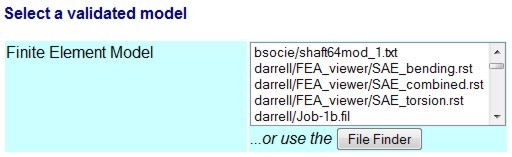
The first step in the process is to select a finite element model for the computation. You can upload a new file from your computer or select from a list of previously uploaded files.

Uploading is a two stage process. First, the file is uploaded to your working directory in eFatigue. You can change your working directory by going to Files in the left sidebar. Once the file is uploaded it is then validated. The validation process consists of reading the entire file to to make sure that it can be read by eFatigue and that it contains all of the information required by the analysis. A list of surface nodes and elements is constructed and linked with the original file. The validation process is only preformed once on each file.
You can also select a model from a list of previously validated files. Clicking on the File Finder will present a list of valid finite element models in your working directory.
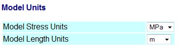
Next the units for the model must be selected.
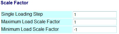
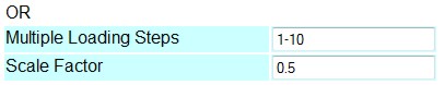
Many finite element models contain only one load step. Fatigue requires cyclic loading. This is acomplished by defining a scale factor for the maximum and minimum load. For example, loads that cycle between zero and the maximum load would have scale factors of Maximum Load Scale Factor = 1 and Minimum Load Scale Factor = 0. Data is scaled as follows: Stress range = ( finite element model stress ) * ( Maximum Load Scale Factor - Minimum Load Scale Factor ) If the model contains several load cases, you can select any one of them for analysis.
Material
At a minimum, the basic strain life properties for the material must be entered. You can also use the Material Property Finder to help you select a material. Frequently the multiaxial fatigue material properties needed for the analysis are not available. eFatigue will make an estimate of these properties.
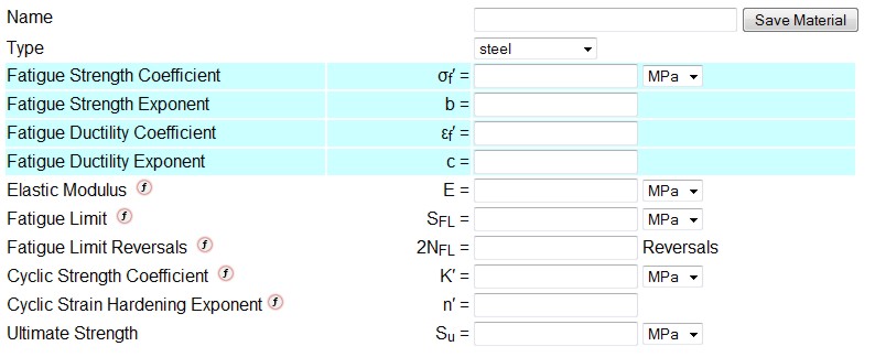
eFatigue uses the following rules for estimating material properties.
| E = |
207,000 MPa for Steel 80,000 MPa for Aluminum |
| 2NFL = | 2E6 |


The ultimate strength can be estimated by noting that the plastic strain at necking is equal to the strain hardening exponent.

Shear Strain Life Curve
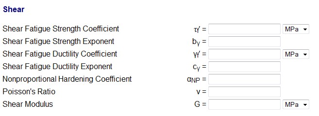
In the absence of test data, an estimate of the shear strain life curve must be obtained. We make the following assumption:
The computed fatigue life for uniaxial loading should be the same for all of the models at the transition fatigue life.
The transition fatigue life, 2Nt, is selected because the elastic and plastic strains contribute equally to the fatigue damage. It can be obtained from the uniaxial fatigue constants.
The Fatemi-Socie model can be employed to determine the shear strain constants.
First we note that the exponents should be the same for shear and tension.
bγ = b
cγ= c
Shear modulus is directly computed from the tensile modulus.
Yield strength can be estimated from the uniaxial cyclic stress strain curve at 0.2% plastic strain.
Normal stresses and strains are computed from the transition fatigue life and uniaxial properties.
Substituting the appropriate value of elastic and plastic Poisson's ratio gives
Separating the elastic and plastic parts of the total strain results in these expressions for the shear strain life constants.
Fatemi-Socie Model Constants

In the absence of test data, a default value of 0.3 is assumed.
Surface Finish
You can enter a surface finish factor directly or select the type of surface from the list. Leaving this field blank will result in a default surface finish factor of 1.

Stress Gradient
Stress gradient effects can be disabled by selecting off. In this case fatigue lives will be computed from the surface stresses.

When stress gradient effects are enabled, which is recommended for the best fatigue estimates, the critical distance may be entered directly. Otherwise it will be estimated from the following equation:
Output Definition
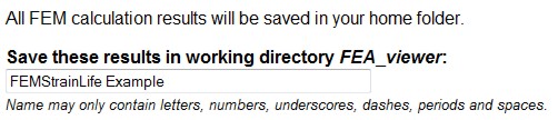
Results of the analysis will be stored in your working directory. This includes all plots and numerical results. You can select your own file name or use the default.
Quick look plots are created for up to 10 nodes after the analysis is completed. These show the sensitivity of the fatigue life at the node to mean stress, material strength, loading and surface finish. You can either leave the list of nodes blank and the most damaging 10 nodes will be plotted or you can specify up to 10 nodes of interest. If you specify more than 10 nodes only the first 10 will be plotted.
A list can be defined using the - range identifier, nodes should be separated by a space. e.g. 1-5 17

eFatigue creates output files in the same format as the input file of fatigue lives or safety factors that can be displayed as contour plots in your FEA viewer. This file will be written to your working directory using the root file name from the input file. You can download this file when the analysis finishes by right clicking on the file name in your working directory. This can be disabled by selecting None from the list.

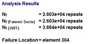
Analysis Results
Results from the eFatigue Strain-Life Analyzer are presented in a series of tables and graphs. The minimum fatigue life is given for both Goodman and Findley models. The expected life is the minimum of the two models.
Contour plots of fatigue lives are automatically produced to show the area where fatigue failures are expected.
Next a bar chart of the fatigue lives for the 10 worst nodes, or the 10 nodes you selected, are given. This chart is based on the minimum of the two fatigue models.
A sensitivity study of the fatigue life on the input variables is then given. The first chart shows how much you would have to change the input variables to get a factor of 2 increase in fatigue life. The second chart gives the same information for a factor of 10. Surface finish factor is often omitted from these charts because you can not change it enough to obtain an increase in life. For example, you can not improve on a surface finish factor that already has a value of 1.
A chart showing the biaxial stress ratio, σ3/σ1 for the critical nodes is given. Uniaxial loading has a value of 0. Torsion is -1 and biaxial tension is 1.
The next two charts give the results of the individual fatigue models.
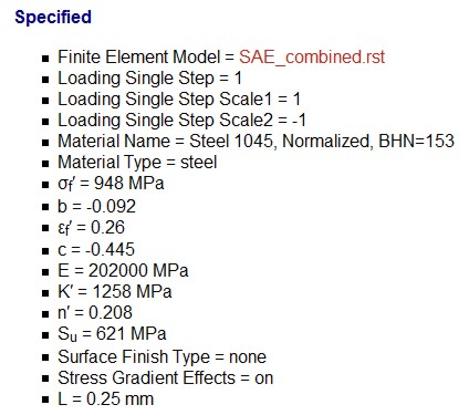
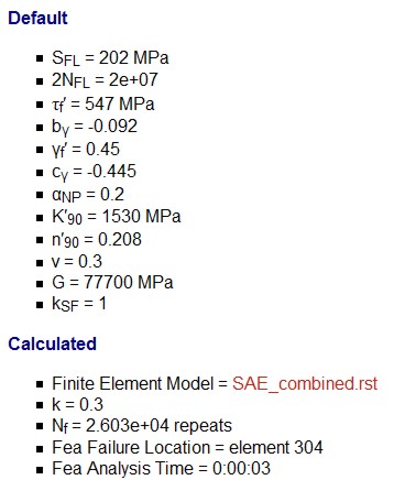
Finally, a listing of the input variables used in the analysis is presented