- Fatigue Technologies
- Constant Amplitude
- Variable Amplitude
- Fatigue Analyzers
- Finders
- Technical Background
- Finite Element Model
- Multiaxial
- Probabilistic
- High Temperature
- Welded Structures
- Cast Iron
- Small Defect √ Area
- Utilities
- Languages
 日本語
日本語eFatigue gives you everything you need to perform state-of-the-art fatigue analysis over the web. Click here to learn more about eFatigue.
Variable Amplitude Strain-Life Technical Background
Strain life analysis can be summarized as a series of steps:
- define applied nominal stresses or strains
- select material properties
- determine stress concentration factor
- use Neuber's rule to compute local stresses and strains
- rainflow count to identify cycles
- sum fatigue damage for each cycle
Go to the Constant Amplitude Technical Background section for a more complete description of the fatigue variables.
In the other fatigue methods, Stress-Life, Crack Growth and Welds, it doesn't make any difference if the loading history is entered as a time history or a rainflow histogram. Both give the same results. Because of cyclic plasticity, some mean stress information is lost in a rainflow histogram.
Here is a simple example with six loading sequences with both zero and non-zero mean strains. In this figure the the initial setup cycle is shown black and the repeated cyclic loading is shown in red.
From the loading histories alone it is imposssible to tell which histories will have zero mean stress. In A the stresses and strains remain elastic and a positive mean stress is produced that is proportional to the strains. In B plastic deformation occurs during the initial loading and the resulting mean stress is zero enen though the mean strain is tensile. A compressive mean stress is procuced in C for a zero mean strain. D is the mirror image of B and E is the mirror image of C. By carefull adjusting the initial loading F it is possible to have both zero mean stress and zero mean strain.
In a rainflow histogram, only strain ranges and mean strains are recorded. This makes it impossible to distinguish between C, E and F. In more complex loading situations it is impossible to distinguish between these three possibilities even if the data has been recorded in a To-From format. As a result, all three possibilities are analyzed and the resulting fatigue lives reported. These represent the maximum possible tensile mean stress effect, no mean stress, and maximum compressive mean stress effect.
Loading History
Several methods may be used to input the loading history. These include Text Boxes, Clipboard and Files. Loading data may be either time histories or histograms.
Text Box input may be used to manually enter a loading history. The loading history can contain several channels, one channel per column. Histograms may also be entered. Histograms must be a square matrix in a To-From format with the same number of rows and columns. The first row and column must contain the values for the bin limits. An example of the histogram format can be found in the files section. Supported File Types
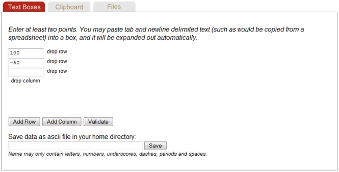
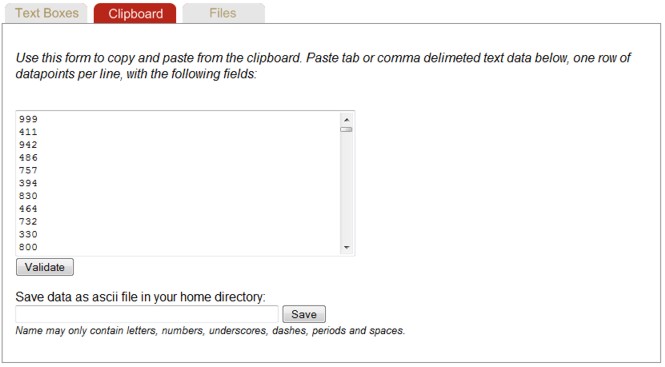
The Clipboard entry is a more convienient way to enter large chunks of data. Data in the clipboard may be edited directly in the clipboard view and is also automatically placed in the text boxes. Similarly, data entered in Text Boxes is available in the clipboard view.
eFatigue supports a number of data file formats. A complete description is found in Supported File Types.
Go to Working With Files if you are unfamiliar with the eFatigue file system.
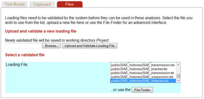
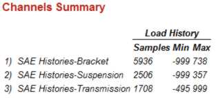
eFatigue uses a file validation process to make sure that the file can be read before conducting any analysis. Key information such as number of channels, maximums and minimums are also obtained from the validation process. This information is always displayed once a file is selected.
Units for the loading history must be selected. The load scale factor defaults to 1 and zero offset to 0 if left blank. Data is scaled as data * scale + offset.
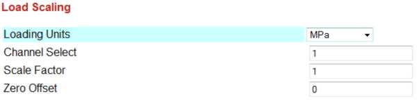
Unscaled data may be plotted with the Plot button.
Materials Data
Materials data entry and defaults are the same as constant amplitude analysis. Go to the Constant Amplitude Technical Background section for a more complete description.
Surface Finish Effects
Surface finish entry and defaults are the same as constant amplitude analysis. Go to the Constant Amplitude Technical Background section for a more complete description.
Stress Concentration
Stress concentration factor entry and defaults are the same as constant amplitude analysis. Go to the Constant Amplitude Technical Background section for a more complete description.
Output File
You can specify a filename for the output results in the Output Definition section. A default filename will be assigned if this is left blank.
Analyze
A new window will appear after the Analysis is started. At this point the analysis is sent to a separate server for processing. You may safely navigate away from this window at this point. If you remain on this page, the analysis results will automatically be displayed when completed. Otherwise the analysis results willl be placed in your working directory. For a very long loading history, you may wish to turn on an email notification by going to your Account page.
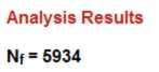
Results
The fatigue life is given first. The number represents the number of times the entire load history can be repeated, not the total number of cycles.
Hysteresis loops for the largest cycles are displayed.
A cumulative exceedance diagram for the cycle ranges is displayed. These diagrams are useful for describing the nature of the loading history and to compare one history with another in terms of stress amplitudes and number of cycles.
Rainflow histograms of the cycles are displayed if the input is a time history. They are displayed in a To_From format. In this format, zero range is along the one of the diagonals and zero mean along the other diagonal.
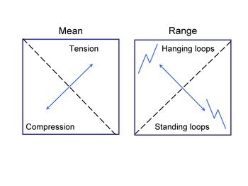
This loading history has a fairly symmetric distribution of hanging and standing cycles. It also has a tensile mean.
The fatigue damage for each bin in the cycle histogram is displayed. Damage for larger cycles will always be more than the damage for an individual smaller cycle. The damage displayed represents the damage for all of the cycles in a bin. In this loading history, most of the damage is done by a small number of high amplitude cycles.
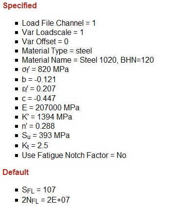
Finally, a listing of all of the input parameters is given with any default parameters that have been used in the analysis.